
We do a lot of document processing at OBLSK. Recently, we dug into architectural drawings, specifically home floor plans. We assumed an AI pipeline would pull the room data out. We were wrong.
The question is how big each room is.
Every number in this post comes from one file, simple_floorplan.dxf. It is a 14-room single-story house, and each room is stored as a closed polyline. One method reads those polylines. The other two read a PNG render of the same file. Nothing else varies.
Each object has a name, a polygon as a list of [x, y] vertices, and an area computed from those vertices with the shoelace formula.
Joining a predicted polygon to a real room needs a rule, and the rule changes the answer. I used centroid containment. A prediction joins a room when the prediction’s centroid falls inside that room’s native polygon. Intersection-over-union would have scored one enormous blob as a partial hit on many rooms. Centroid containment scores it as exactly one wrong room.
Results
I scored three readings of one file against the same 14-room schedule and the same join rule.
| Method | Input | Found |
|---|---|---|
| Native DXF polylines | CAD entities | 14 of 14 |
| Gemini 3.8 Flash | PNG render | 12 of 14 |
| CubiCasa5K | PNG render | 0 of 14 |
Finding rooms with Gemini
I started with a general-purpose multimodal LLM, Gemini 3.8 Flash.
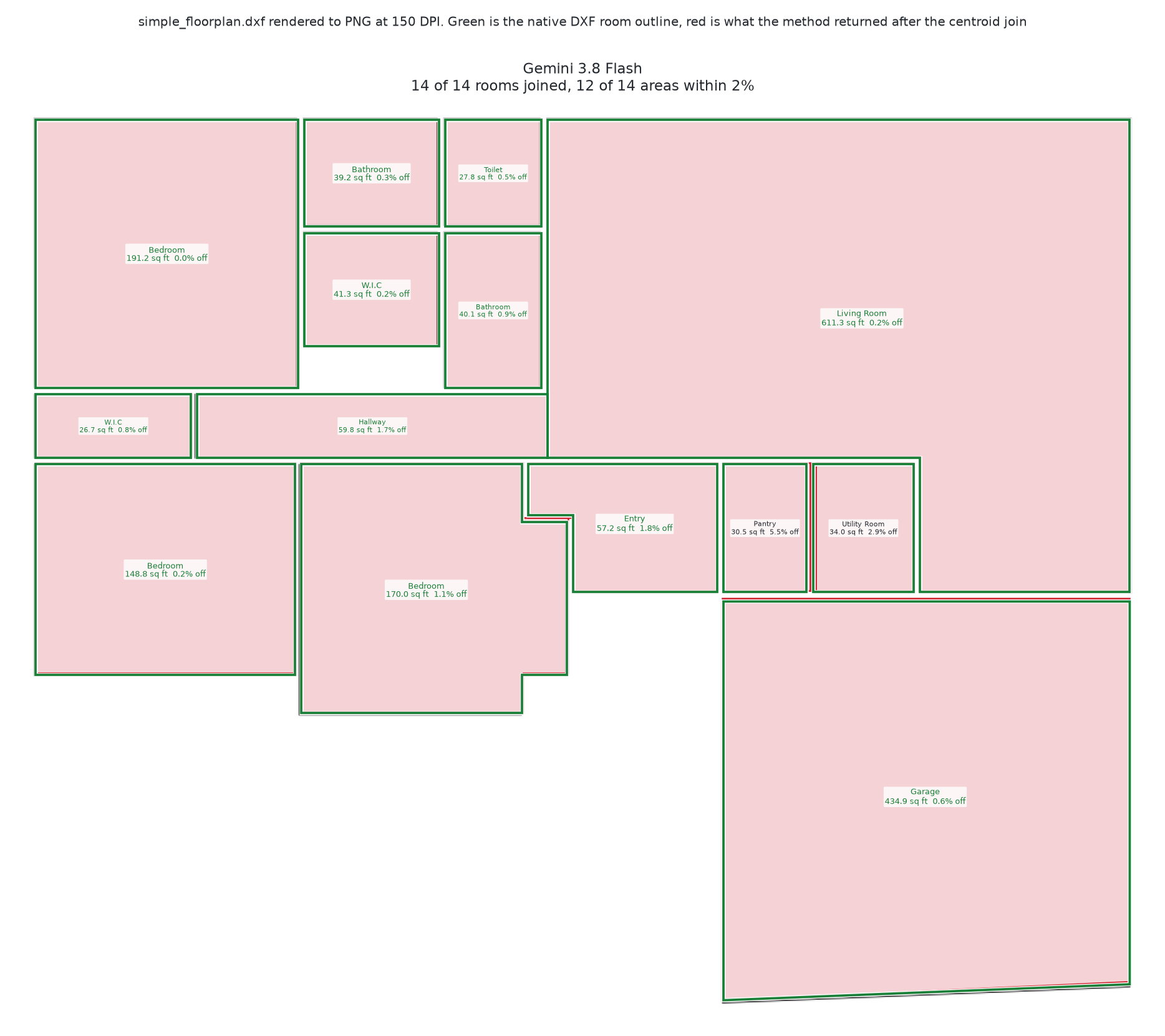
Gemini found all 14 rooms. It placed every centroid inside the correct room.
A few areas were off. The Living Room is 612.3 square feet and Gemini called it 611.3, off by 0.2 percent. The Entry is 56.2 and came back 57.2, off by 1.8 percent. The Pantry is 28.9 square feet and came back 30.5, off by 5.5 percent. The Utility Room is 35.0 and came back 34.0, off by 2.9 percent.
Finding rooms with CubiCasa
Next, I tested CubiCasa5K, a neural network trained on architectural floor plans. I expected it to beat a general-purpose model.
It returned a single region labeled “Other rooms” covering most of the drawing. That blob measures 1,514.6 square feet, and the room its centroid lands in is a 168.2 square foot bedroom. It is nine times too large. One room joined, zero areas within tolerance, and thirteen rooms never located at all.
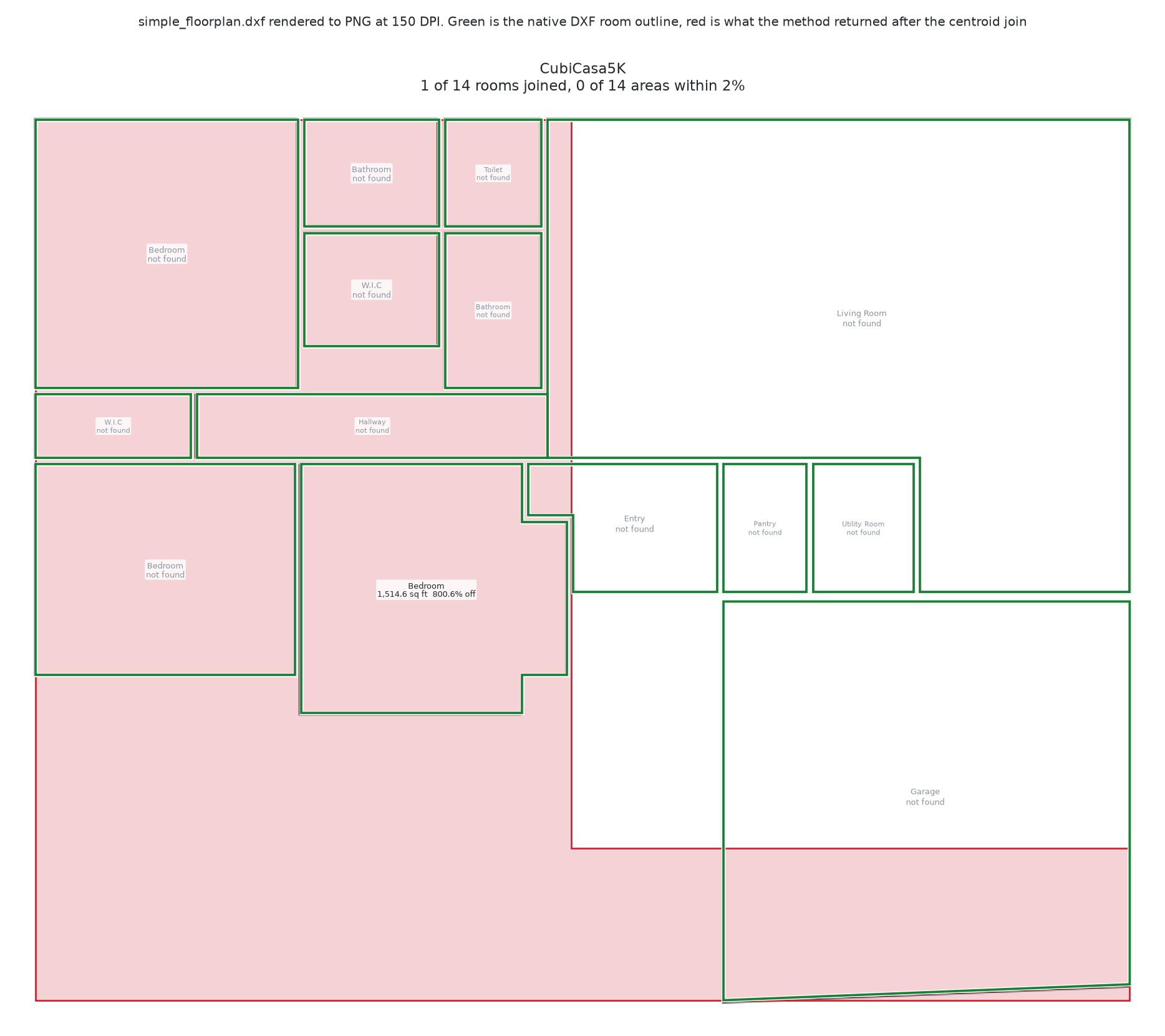
Training distribution explains the failure. CubiCasa learned from marketing-style floor plans with shaded rooms, furniture symbols, and filled wall cavities. A bare CAD line drawing with no fill is a different visual domain. The words “floor plan” in the model name do not mean it can read a CAD wireframe.
Native CAD geometry
simple_floorplan.dxf holds 14 LWPOLYLINE entities, one closed polyline per room. A companion CSV gives each room a name and a coordinate point. We apply the shoelace formula to each polyline for its exact area, then join each CSV point to the polyline that contains it.
Native geometry recovered 14 of 14 rooms, all 14 names, and all 14 areas with zero measurement error. That is the schedule every other method was scored against: a 612.3 square foot Living Room, a 432.2 square foot Garage, three bedrooms at 191.3, 168.2, and 148.5, down to a 26.9 square foot walk-in closet, totalling 1,909 square feet. It is also the green outline in all three figures above.
simple_floorplan.dxf, its room mapping CSV, and the construction sheet that supplied the scale all come from CCWI/building-plan-viewer under MIT. That sheet originates in jscad/sample-files, also MIT. Having the room polygons published alongside the drawing enabled this comparison without manual labeling.
What this does not prove
simple_floorplan.dxf is small, clean, and single-story, and its rooms are already closed polylines. It is the easiest input in this comparison. How these three methods behave on a real construction sheet is a separate measurement, and that measurement is not in this post.
The scale is derived, not measured off a physical print. A companion sheet’s dimension style declares architectural units, and two of that sheet’s overall dimensions match the room-polygon span once exterior walls are subtracted. The scale is still an inference from the file, not a survey of the building. The comparison does not depend on the scale, because relative error cancels the unit.
This render has no text, so it does not test label reading. Gemini 3.8 Flash located all fourteen rooms and got 12 areas within 2 percent on the easiest drawing in the set. It still did not produce a 14-row schedule with zero measurement error, and this is one model on one PNG.
If you are evaluating a vendor on document work, the more general version of this is on our evaluation guide, which asks for denominated failures on hard document types rather than a single accuracy percentage.
Score against the native schedule
Build the native schedule first. Score every other reading of the same file against it, with the same join rule and the same tolerance. A miss is one row, with a room name and a number.
If the pipeline has to return numbers taken from the geometry, read the geometry. A PNG or a PDF is a picture of that geometry, and flattening it to pixels discards the exact vectors. Sometimes the only file available is the PNG or the PDF.
My thanks to Isaac Flath, whose writing on parsing text, tables, and structure out of PDFs prompted me to measure the adjacent case where the payload is closed geometry rather than prose.